The MATLAB function holo is copyrighted by John C. Polking of Rice University. It is not in the public domain. However it is made available free to all users who use it exclusively for educational purposes. It is requested that all who use holo register that fact by send email to John C. Polking, (polking@rice.edu). It is not free for anyone who will use it in any way for commercial uses.
To download the file shift click here.
To use the program holo, first start MATLAB, and then enter
>> holo
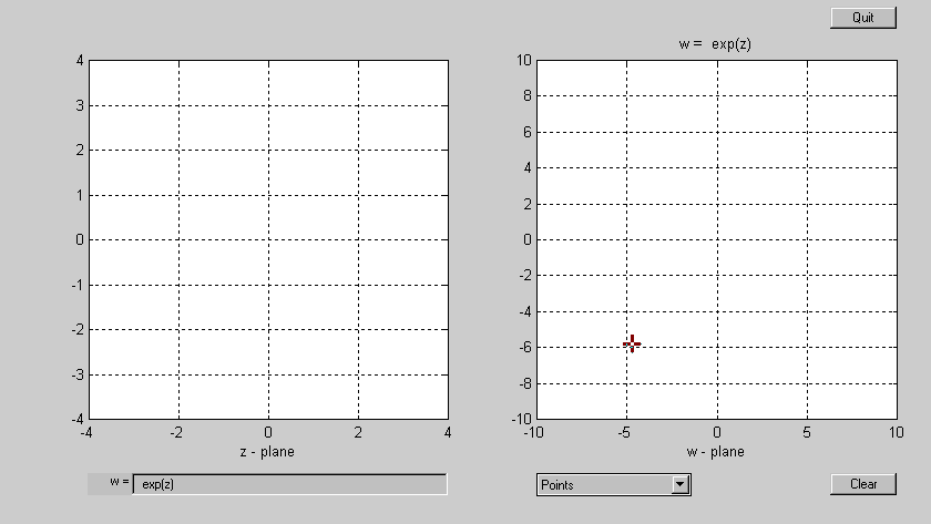
at the MATLAB prompt. From now on you can forget MATLAB, and
just deal with the new window that appears:
You will notice that w = exp(z) is the default holomorphic function. This can be changed to whatever the user wants.
You will also notice a button labeled "Points". If you click the
mouse on it, you will discover that it is a popup menu, and that there
are five modes available. To use the default "Points" mode, simply
click the mouse on the z-plane. The point and its image in the w-plane
will be plotted in the same color.
In the other modes a more complicated mouse action is required.
You must depress the mouse at a point, and then drag it to another point
before releasing it. In the "Lines" mode, as you drag the mouse you
will see a line from the initial point to the new one in the z-plane
and its image in the w-plane. When you release the mouse the two
curves will again both have the same color. In the "Circles"
mode, as you drag the mouse in the z-plane you will get a circle with its
center at the initial point and passing through the through the second
point, and you will see its image in the w-plane. Once more, when
the mouse button is released both curves will be plotted in the same color.
In the "Rectangular grid" mode, dragging the mouse will outline a rectangle in the z-plane together with its image in the w-plane. When the mouse is released you will get a rectangular grid in the z-plane and its image inthe w-plane. the corresponding parts of the grids are plotted in the same colors. The "Polar grid" mode acts in the same manner, but results in a circular grid and its image.
When the figure get too complicated, click on the "Clear" button to erase everything.
When you are finished, click on the "Quit" button.
If you want to print the figure, simply enter print at the MATLAB prompt. If instead you use print -noui the figure will print without any of the control boxes.
You can change the function by double-clicking in the edit box, and then entering what you want. The text that was originally there will be deleted. Make sure it is a function of z. You are not allowed to choose your own variables.
The options for changing the limits on the two planes are also fairly straightforward. However, it will be noticed that the user is allowed to enter only the complex corner at the lower left hand corner and the real increment. The imaginary increment will be the same as the real increment with the result that each plane is kept square and conformality is maintained.
This might cause problems of interpretation for some users of holo. For example, enter the function w = sqrt(z^2). Almost any reasonable person who was not into complex analysis might think that this should be the same as the identity map w = z. However, if you try this in holo you will not get the identity map. The square root function acts on the argument of z^2, and the result is the identity in half of the plane and the negative of the identity in the other.
The fact that MATLAB is very precise in its definition of every individual
function can lead to surprises like this with composite functions.
However, this in itself can be a learning experience for students new to
the subject.